
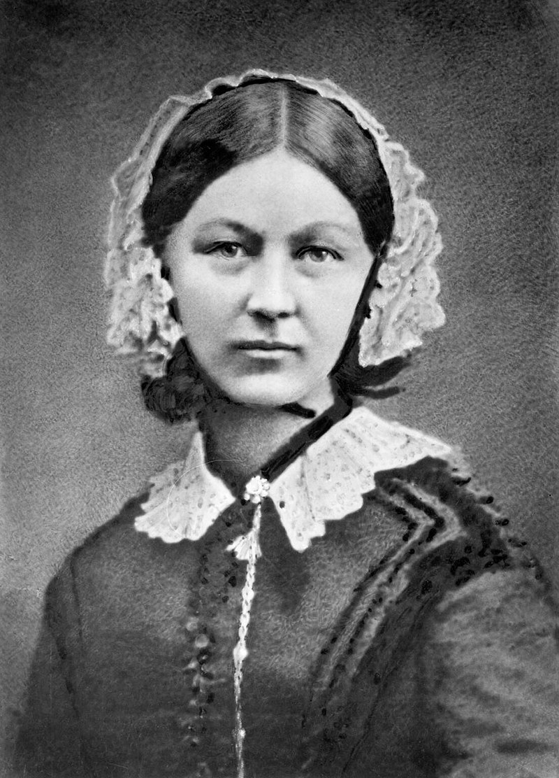
| Cause | Deaths |
|---|---|
| Preventable disease | 14476 |
| Wounds | 1758 |
| Other | 1748 |
5. JASP & Visualization
9 September 2026
Why JASP?
- User-friendly, intuitive interface
- Open-source (free)
- Reproducible analyses (easy to share)
- Better than IBM’s SPSS for transparency and workflow
- Integrates with R for advanced users

Origin
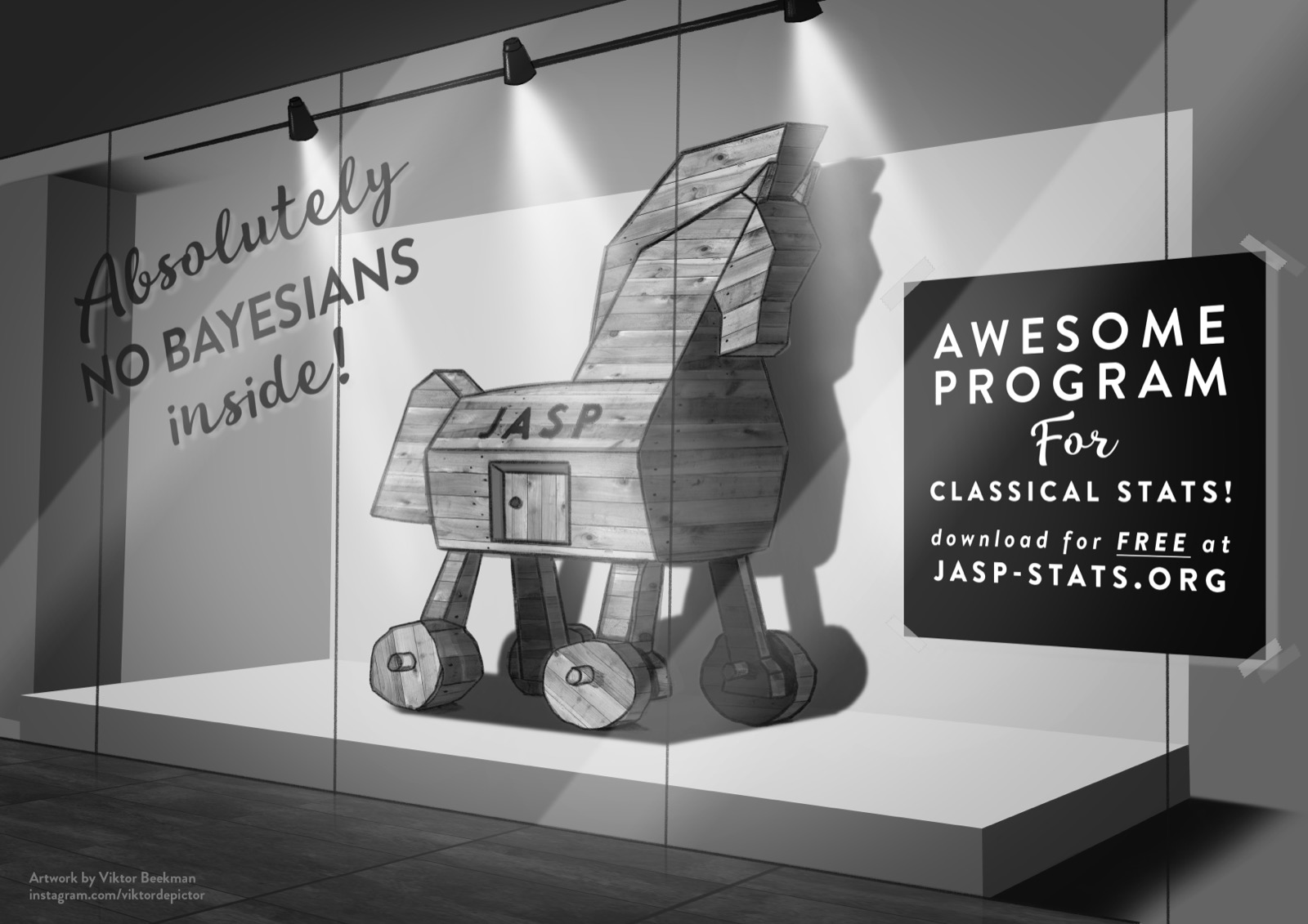
Artwork by Viktor Beekman, via Bayesian Spectacles
The start-up window
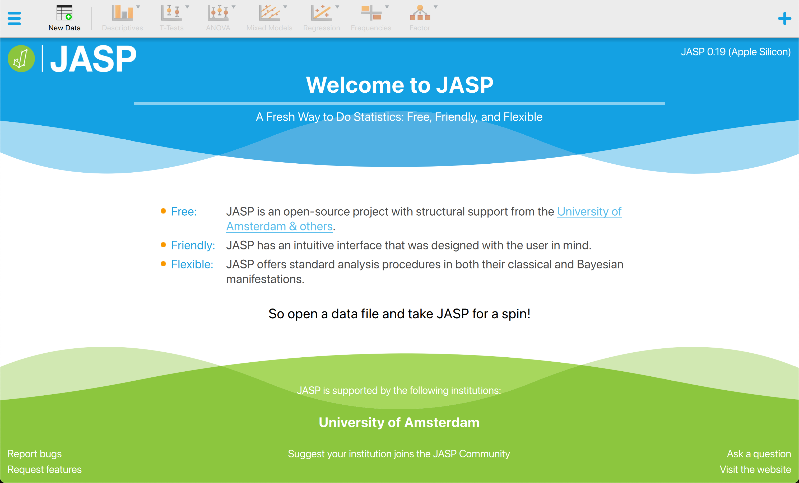
Two buttons
The hamburger button  :
:
- Open files (from computer, the Open Science Framework, or the JASP data library)
- Adjust settings (e.g., dark mode, language, how to display results)
- Save/export data/results
The module button  :
:
- Add modules to the top ribbon bar
- Update modules
The data library
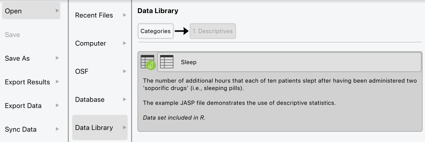
Loading Data in JASP
- Click Open > select your file
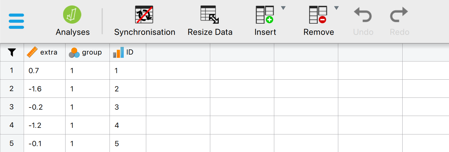
- Data appears in spreadsheet view
Variable settings
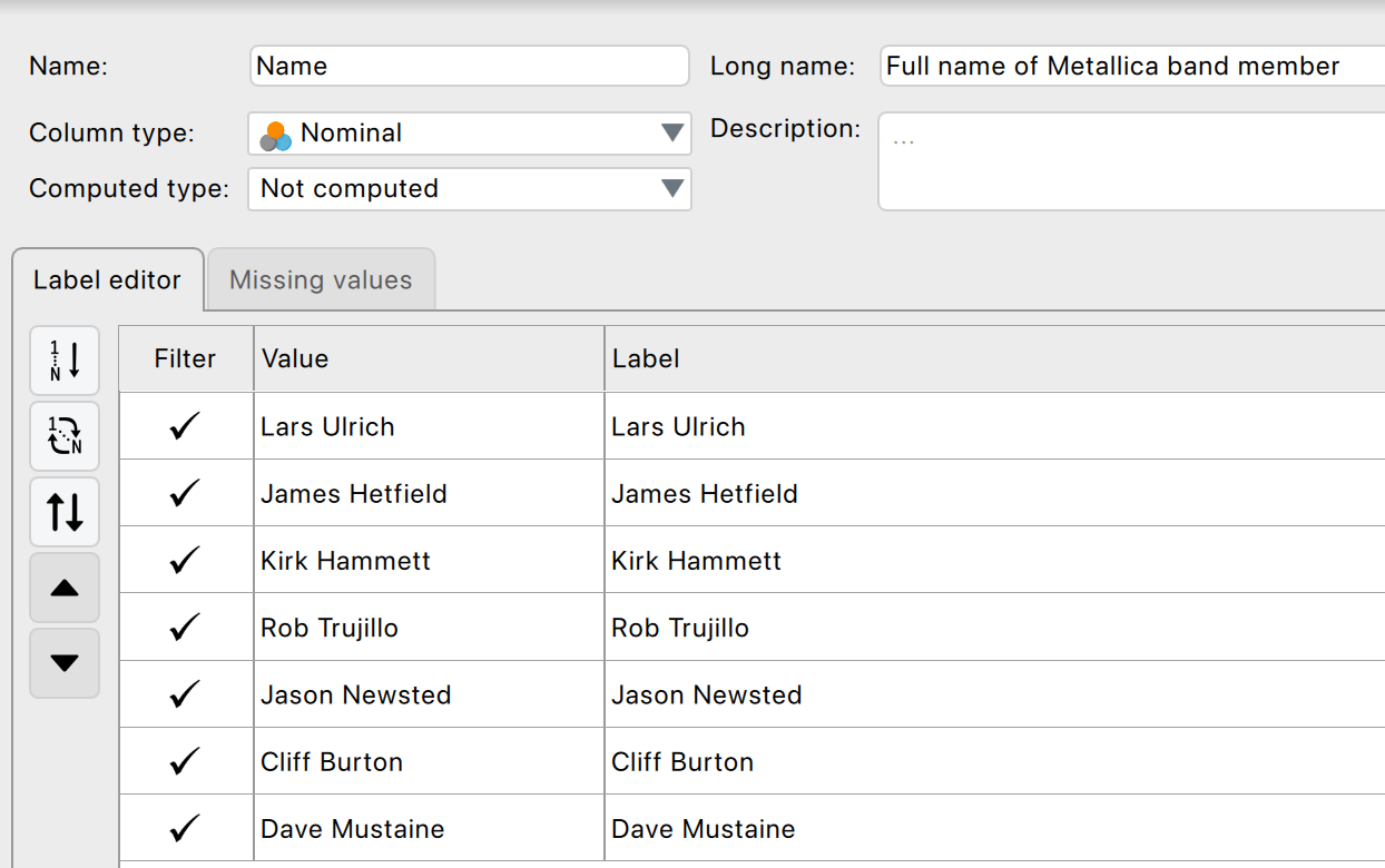
Doubleclick a column name to open its settings. The measurement level you set here decides how JASP treats your variable.
Ordinal variables
Computing a new variable
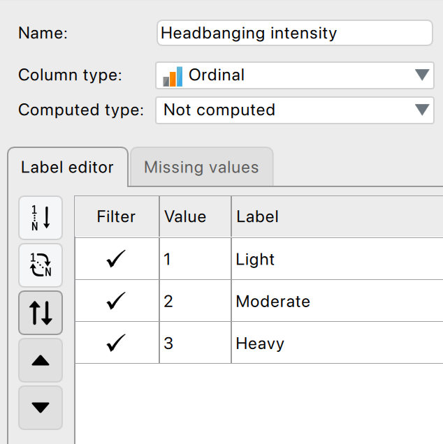
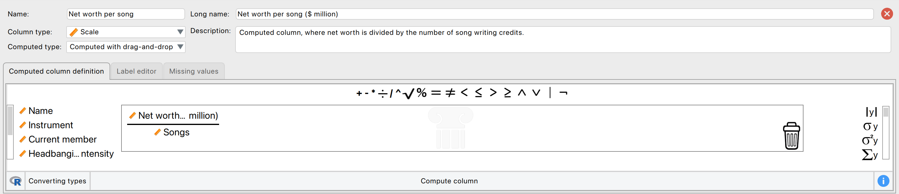
Drag and drop, no syntax required.
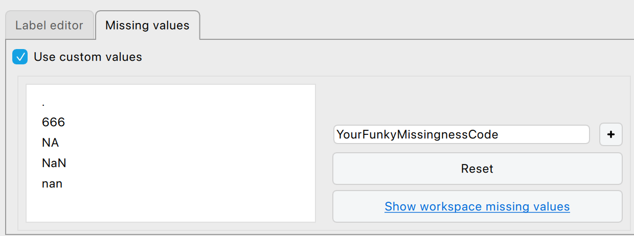
Missing values
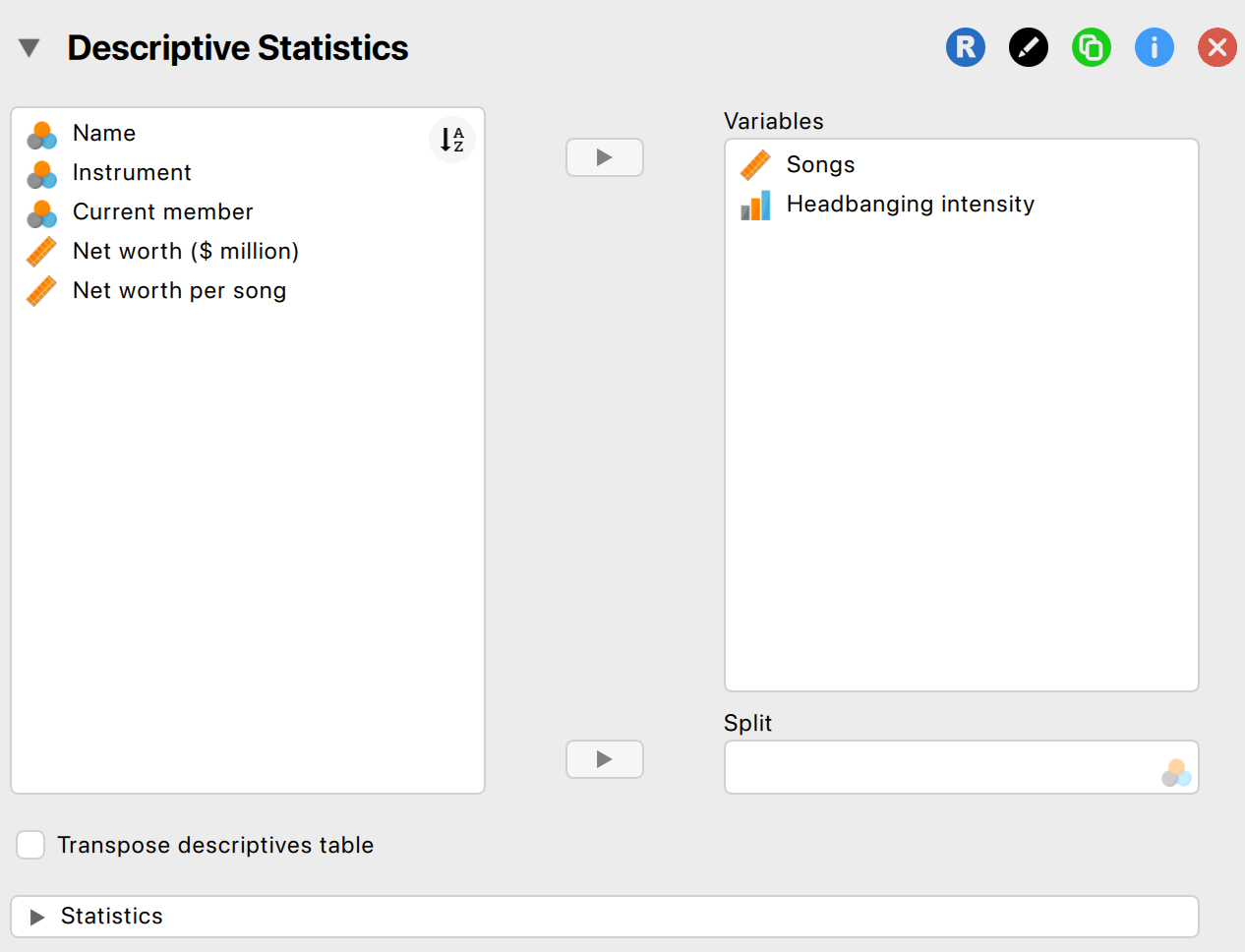
Descriptive Statistics in JASP
- Go to Descriptives > select variables
- Options: mean, median, SD, min, max, quartiles
- Output updates instantly
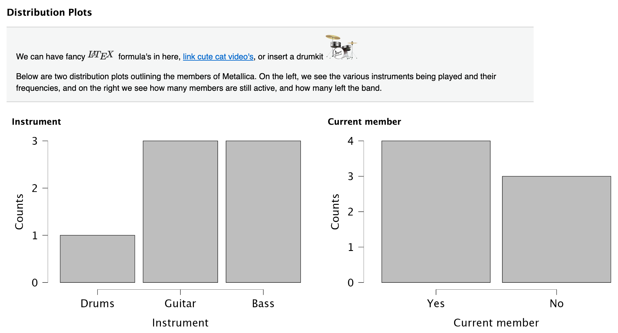
Annotated output
Getting help
- JASP Video Library
- The book
![]()
Why Visualize Data?
- Quick overview of the data
- Spot patterns, outliers, or errors
- Invite the reader
Why Visualize Data?
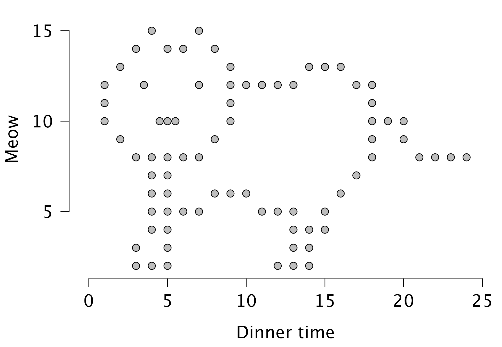
Figure 5.15 Catterplot
Scutari, 1854
- Military hospital, Crimean War
- Recorded every death and its cause
- Two years of counting:
- Infection killed far more than the enemy did
- Sanitary Commission arrived March 1855
- Later the first woman elected to the Statistical Society
The diagram
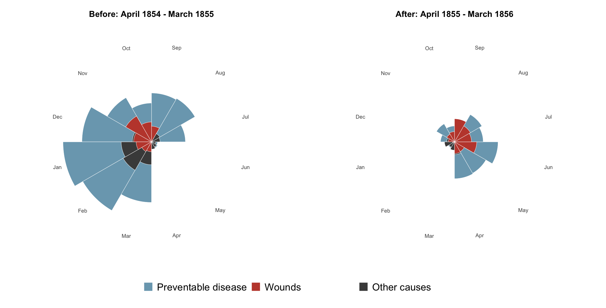
Each wedge is a month; its area is the death rate.
Boxplots: Visualizing Spread and Outliers
- Shows median, quartiles, and outliers
- Useful for comparing groups
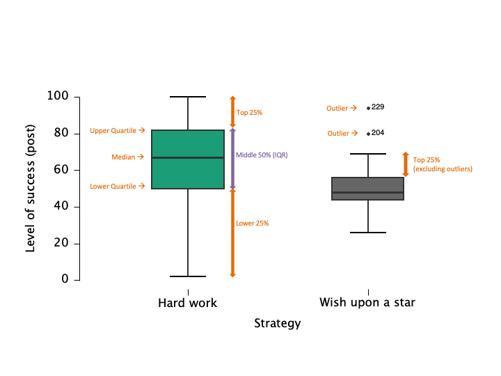
Figure 5.9 Boxplots
Raincloud plots: Boxplots + Raw Data
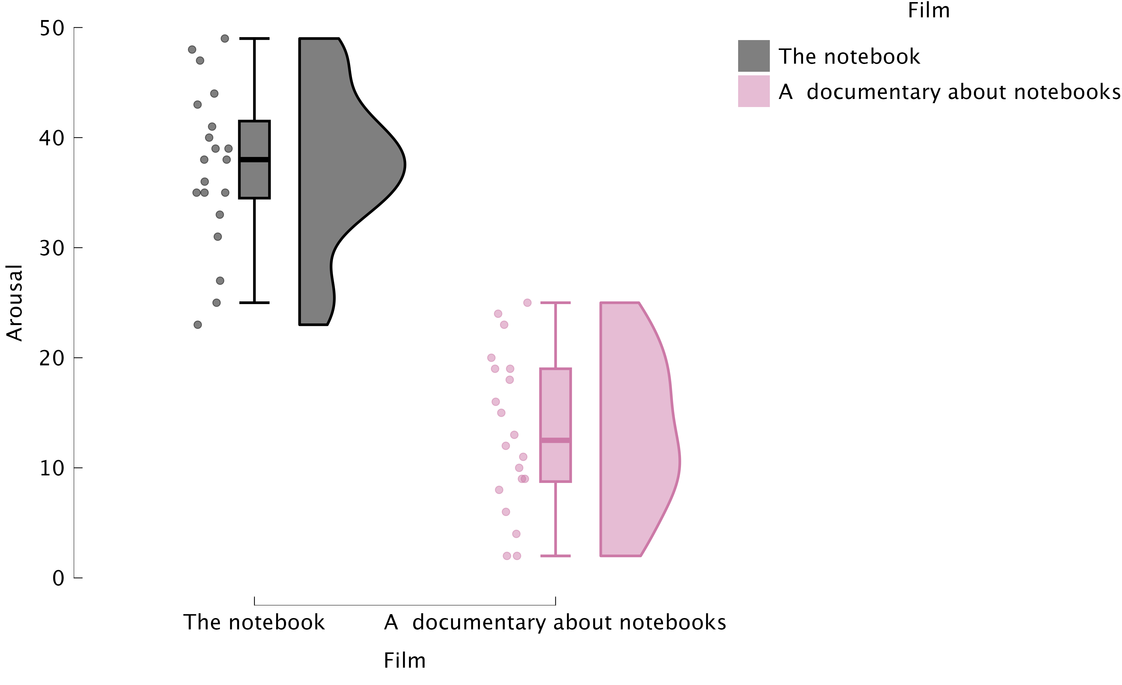
Figure 5.11 Raincloud plots
Labels and axes
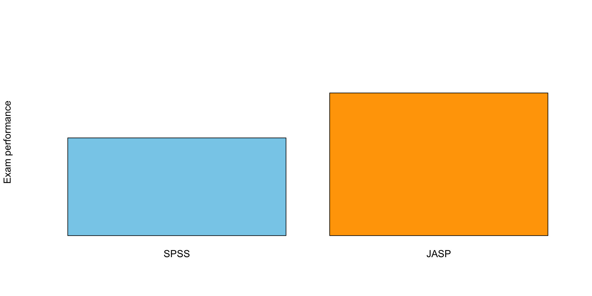
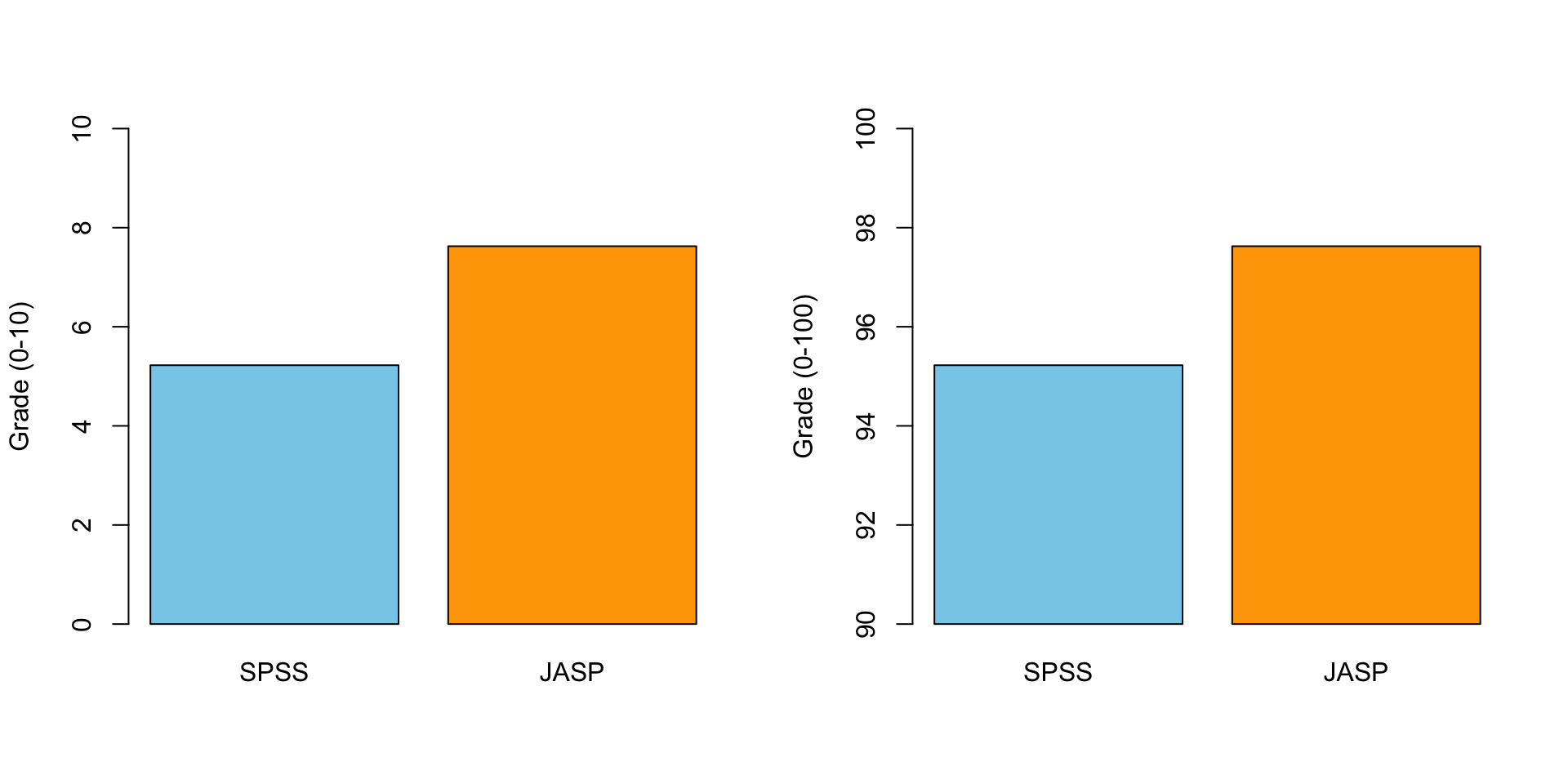
Scale Matters
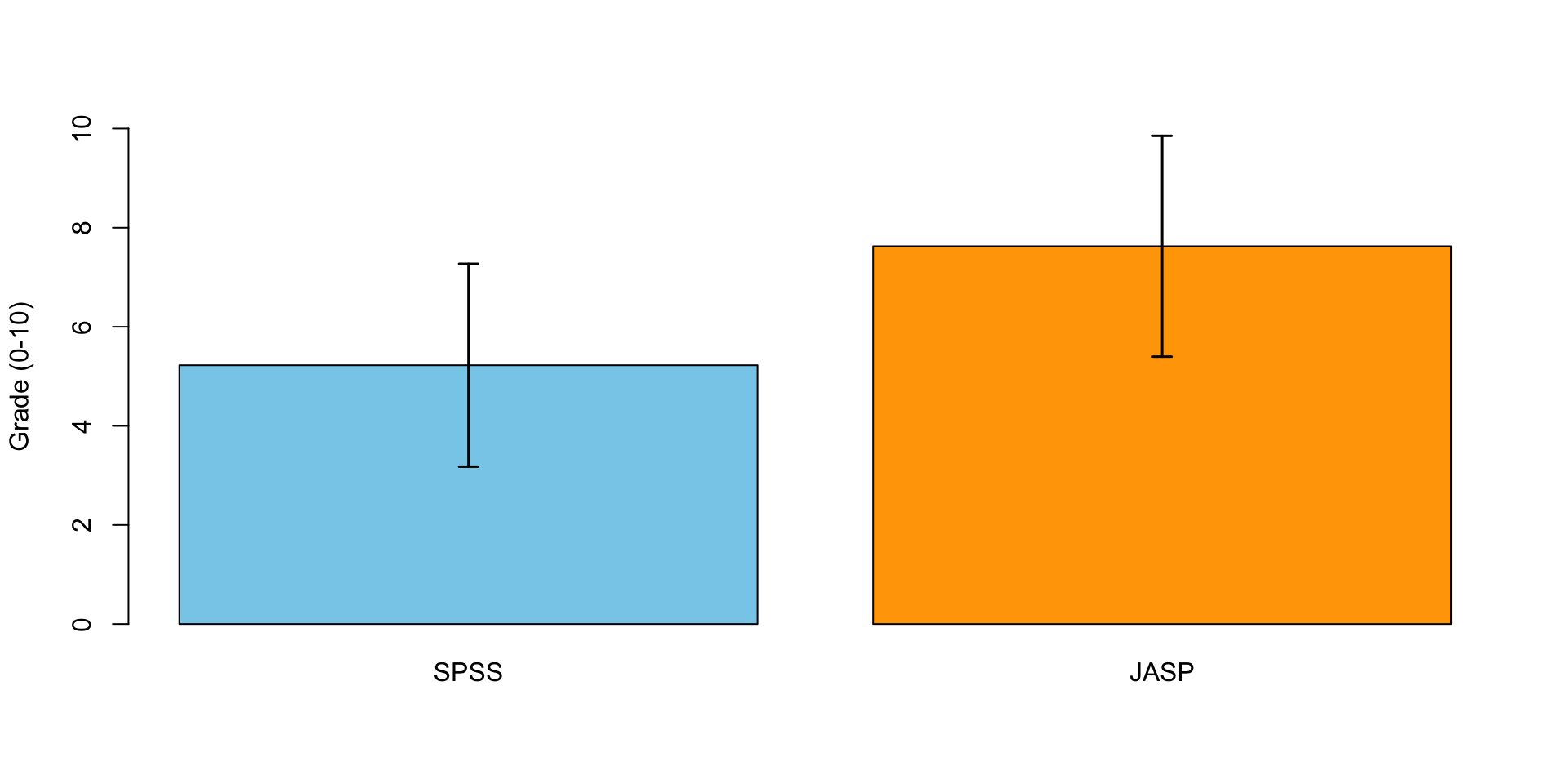
Error Bars!
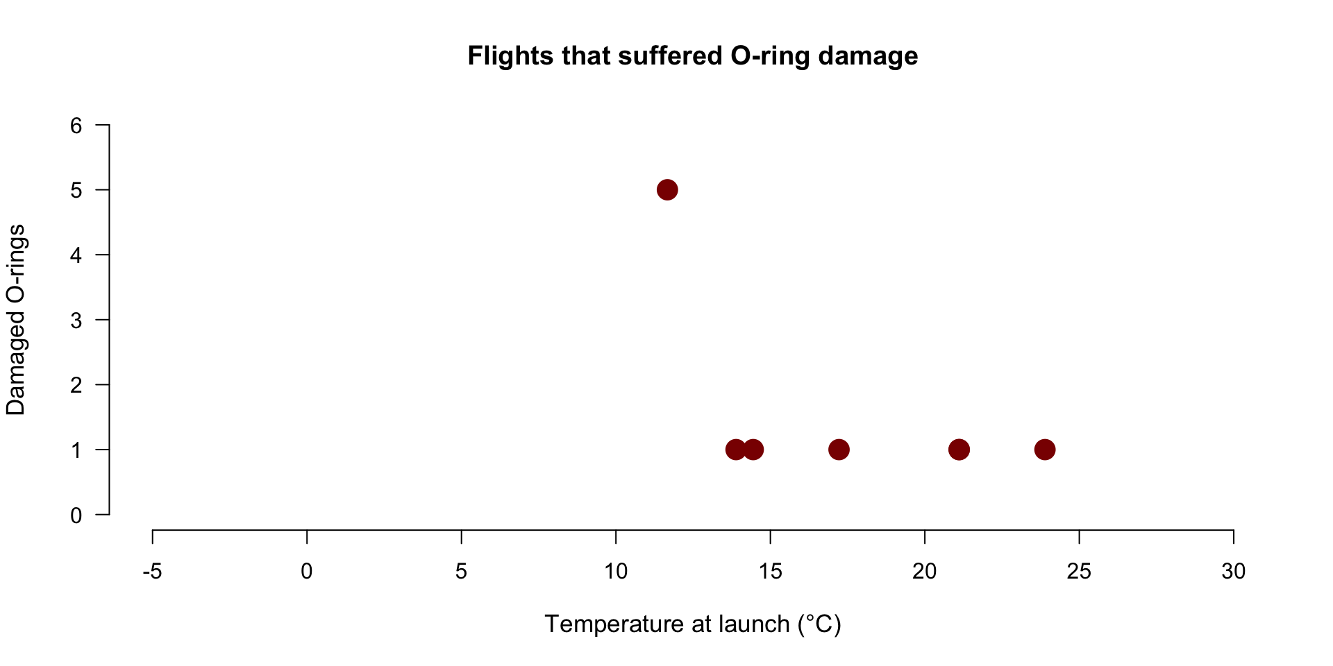
The evidence they reviewed
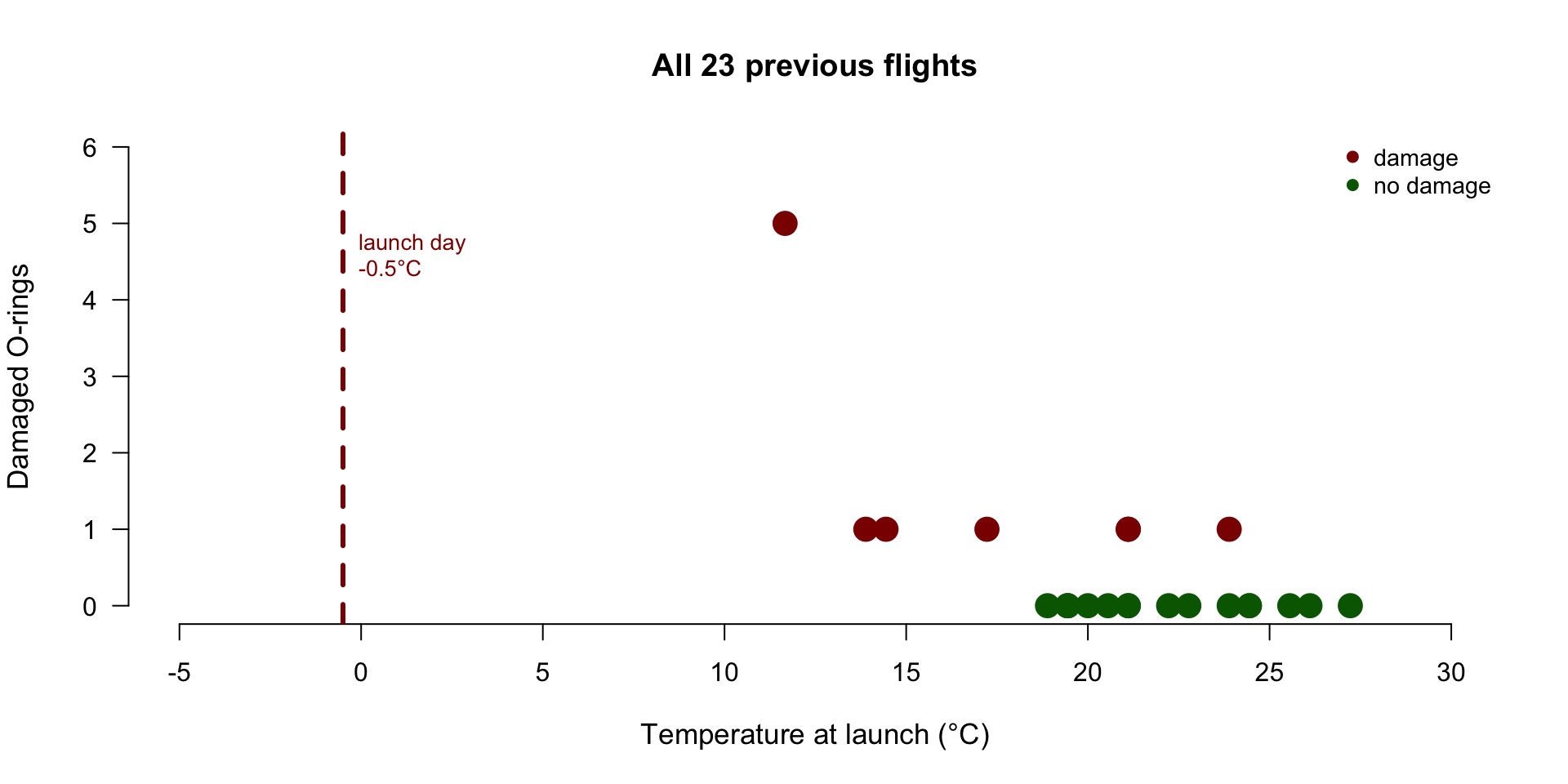
The flights that were excluded
Contact

